🔥알림🔥
① 테디노트 유튜브 -
구경하러 가기!
② LangChain 한국어 튜토리얼
바로가기 👀
③ 랭체인 노트 무료 전자책(wikidocs)
바로가기 🙌
④ RAG 비법노트 LangChain 강의오픈
바로가기 🙌
⑤ 서울대 PyTorch 딥러닝 강의
바로가기 🙌
Python 과 Tensorflow로 Mnist 글자인식 구현하기
이번 포스팅에서는 Mnist 데이터를 땡파이썬으로 구현해봄과 동시에 Tensorflow 를 활용하여 구현해 보겠다.
우선, 첫번째로는 땡 Python 코드로 글자 인식을 구현해 보는 것이고,
두번째로는 Tensorflow를 이용하여 깔끔하게 구현해 보겠다.
이번 구현의 핵심은 Multi-class Classification 에 있다.
Multi-class Classification이란, 주어진 데이터를 Multi-class로 분류,
다시 말해서, 무작위로 주어진 픽셀값들의 학습을 통해 씌여진 글자가 0 ~ 9로 분류하는 머신러닝 알고리즘의 구현이다.
Mnist란?
Mnist는 Mixed National Institute of Standards and Technology database의 약어로 손글씨 숫자 이미지들을 모아놓은 데이터이다. 28 * 28 의 매트릭스안에 색상 (밝기)값으로 정의 되어 있다.
Mnist Data Loading
Mnist 데이터를 받아와야하는데, 여러 경로로 데이터를 얻을 수 있지만, 이번에는 keras.datasets에 있는 mnist 를 활용했다.
from keras.datasets import mnist

((x_train, y_train), (x_test, y_test)) = mnist.load_data()

print(x_train.shape, x_test.shape)
print(y_train.shape, y_test.shape)

## (60000, 28, 28) (10000, 28, 28)
## (60000,) (10000,)
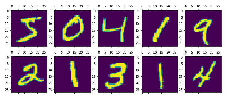
Mnist Data를 Matplotlib으로 그려보기
figure = plt.figure()
figure.set_size_inches(12, 5)

axes = []
for i in range(1, 11):
    axes.append(figure.add_subplot(2, 5, i))

for i in range(10):
    axes[i].matshow(t[i])
결과
Python코드로 Mnist 글자 인식 구현
activation function으로는 sigmoid를 활용해 보았다.
주로, multi-class classification에는 activation function 으로 softmax함수와 cross-entropy를 사용하나, 이번 구현에서는 sigmoid 로 구현해 보았다.
Sigmoid
def sigmoid(x):
    return 1 / (1+np.exp(-x))
Cross-entropy
def cross_entropy(actual, predict, eps=1e-15):
    actual = np.array(actual)
    predict = np.array(predict)
    clipped_predict = np.minimum(np.maximum(predict, eps), 1 - eps)
    loss = actual * np.log(clipped_predict) + (1 - actual) * np.log(1 - clipped_predict
    return -1.0 * loss.mean()
[1단계] x_train 데이터를 flatten 시키기
print(x_train.shape)
x_train = x_train.reshape(60000, 28 * 28)
print(x_train.shape)

print(x_test.shape)
x_test = x_test.reshape(10000, 28 * 28)
print(x_test.shape)

## (60000, 28, 28)
## (60000, 784)
## (10000, 28, 28)
## (10000, 784)
[2단계] y_train 데이터를 one hot encoding 시키기
y_train_hot = np.eye(10)[y_train]
[3단계] 학습 구현
## 편의상 x_train데이터를 X로 copy
X = x_train.copy()

## epoch횟수 / learning_rate 정의
num_epoch = 100
learning_rate = 0.1

## weight / bias 정의
W = np.random.uniform(low=-1.0, high=1.0, size=(784, 10))
b = np.random.uniform(low=-1.0, high=1.0, size=10)

for epoch in range(num_epoch):
    hypothesis = np.matmul(X, W) + b
    activated_hypothesis = sigmoid(hypothesis)

    predict = np.argmax(activated_hypothesis, axis=1)
    accuracy = (predict == y_train).mean()

    loss = cross_entropy(activated_hypothesis, y_train_hot)

    if epoch % 10 == 0:
        print(epoch, accuracy, loss)

    if accuracy > 0.80:
        break

    gradient = learning_rate * (np.matmul(X.T, (activated_hypothesis - y_train_hot)))
    bias_gradient = learning_rate * (activated_hypothesis - y_train_hot).mean(axis=0)

    W -= gradient
    b -= bias_gradient

print(epoch, accuracy, loss)

## 0 0.0899 21.76480412531003
## 10 0.7287 2.3506651592952474
## 20 0.7918666666666667 1.8564116855549249
## 30 0.7642 2.0453374304541296
## 32 0.8146833333333333 1.7550393560164779
epoch이 32에 도달하는 순간 accuracy는 81.46833에 도달하여 break 되었다.
Tensorflow로 구현
[1단계] Variable과 one_hot 인코딩 하기
import tensorflow as tf

x_train.shape, y_train.shape
## ((60000, 784), (60000,))

y_train = y_train.reshape([-1, 1])

x_data = tf.Variable(x_train, dtype=tf.float32)
y_data = tf.Variable(y_train, dtype=tf.float32)

y_data_hot = tf.one_hot(y_train.astype(np.float32), 10)

x_train.shape, y_train.shape
## ((60000, 784), (60000, 1))
[2단계] 학습 구현
X = tf.placeholder(tf.float32, shape=[None, 28 * 28])
Y = tf.placeholder(tf.float32, shape=[None, 1])

W = tf.Variable(tf.random_normal([28 * 28, 10], name='weight'))
b = tf.Variable(tf.random_normal([10]))

logit = tf.matmul(X, W) + b
hypothesis = tf.nn.softmax(logit)

cost_i = tf.nn.softmax_cross_entropy_with_logits_v2(logits=logit, labels=y_data_hot)
cost = tf.reduce_mean(cost_i)

optimizer = tf.train.GradientDescentOptimizer(learning_rate=0.01)
train = optimizer.minimize(cost)

sess = tf.Session()
sess.run(tf.global_variables_initializer())

for epoch in range(num_epoch * 10):
    _, cost_val = sess.run([train, cost], feed_dict={X:x_train, Y:y_train})
    if epoch % 10 == 0:
        print(cost_val)

## ...
## 57.651573
## 55.606205
## 59.267708
## 221.46333
## 68.92298
## 57.586174
## 54.94789
[3단계] 결과 검증
prediction = tf.argmax(hypothesis, 1)
correct_prediction = tf.equal(prediction, tf.argmax(y_train_hot, 1))
accuracy = tf.reduce_mean(tf.cast(correct_prediction, tf.float32))

acc = sess.run(accuracy, feed_dict={X: x_train})
acc

## 0.9092
약 90.92%의 높은 정확도를 달성했다.
참고로, epoch은 python으로 구현한 epoch보다 10배 더 돌렸으며, 성능의 비교를 목적으로 구현함이 아니였기 때문에, 얼마나 성능이 올라갈까? 라는 필자의 궁금증때문에 epoch 을 더 많이 돌렸다.
참고 (Reference): 김성훈 교수님의 “모두를 위한 딥러닝 시즌1”을 참고하여 Tensorflow를 구현하였습니다.
댓글남기기